The following is a guest post by Stefan Troost, he describes the work he did in his bachelor thesis:

In this project we have used the RPython infrastructure to generate an RPython JIT for a less-typical use-case: string pattern matching. The work in this project is based on Parsing Expression Grammars and LPeg, an implementation of PEGs designed to be used in Lua. In this post I will showcase some of the work that went into this project, explain PEGs in general and LPeg in particular, and show some benchmarking results.

Parsing Expression Grammars

Parsing Expression Grammas (PEGs) are a type of formal grammar similar to context-free grammars, with the main difference being that they are unambiguous. This is achieved by redefining the ambiguous choice operator of CFGs (usually noted as |) as an ordered choice operator. In practice this means that if a rule in a PEG presents a choice, a PEG parser should prioritize the leftmost choice. Practical uses include parsing and pattern-searching. In comparison to regular expressions PEGs stand out as being able to be parsed in linear time, being strictly more powerful than REs, as well as being arguably more readable.

LPeg

LPeg is an implementation of PEGs written in C to be used in the Lua programming language. A crucial detail of this implementation is that it parses high level function calls, translating them to bytecode, and interpreting that bytecode. Therefore, we are able to improve that implementation by replacing LPegs C-interpreter with an RPython JIT. I use a modified version of LPeg to parse PEGs and pass the generated Intermediate Representation, the LPeg bytecode, to my VM.

The LPeg Library

The LPeg Interpreter executes bytecodes created by parsing a string of commands using the LPeg library. Our JIT supports a subset of the LPeg library, with some of the more advanced or obscure features being left out. Note that this subset is still powerful enough to do things like parse JSON.

Operator	Description
lpeg.P(string)	Matches string literally
lpeg.P(n)	Matches exactly n characters
lpeg.P(-n)	Matches at most n characters
lpeg.S(string)	Matches any character in string (Set)
lpeg.R(“xy”)	Matches any character between x and y (Range)
pattern^n	Matches at least n repetitions of pattern
pattern^-n	Matches at most n repetitions of pattern
pattern1 * pattern2	Matches pattern1 followed by pattern2
pattern1 + pattern2	Matches pattern1 or pattern2 (ordered choice)
pattern1 - pattern2	Matches pattern1 if pattern2 does not match
-pattern	Equivalent to ("" - pattern)

As a simple example, the pattern lpeg.P"ab"+lpeg.P"cd" would match either the string ab or the string cd.

To extract semantic information from a pattern, captures are needed. These are the following operations supported for capture creation.

Operation	What it produces
lpeg.C(pattern)	the match for pattern plus all captures made by pattern
lpeg.Cp()	the current position (matches the empty string)

(tables taken from the LPeg documentation)

These patterns are translated into bytecode by LPeg, at which point we are able to pass them into our own VM.

The VM

The state of the VM at any point is defined by the following variables:

• PC: program counter indicating the current instruction
• fail: an indicator that some match failed and the VM must backtrack
• index: counter indicating the current character of the input string
• stackentries: stack of return addresses and choice points
• captures: stack of capture objects

The execution of bytecode manipulates the values of these variables in order to produce some output. How that works and what that output looks like will be explained now.

The Bytecode

For simplicity’s sake I will not go over every individual bytecode, but instead choose some that exemplify the core concepts of the bytecode set.

generic character matching bytecodes

• any: Checks if there’s any characters left in the inputstring. If it succeeds it advances the index and PC by 1, if not the bytecode fails.

• char c: Checks if there is another bytecode in the input and if that character is equal to c. Otherwise the bytecode fails.

• set c1-c2: Checks if there is another bytecode in the input and if that character is between (including) c1 and c2. Otherwise the bytecode fails.

These bytecodes are the easiest to understand with very little impact on the VM. What it means for a bytecode to fail will be explained when we get to control flow bytecodes.

To get back to the example, the first half of the pattern lpeg.P"ab" could be compiled to the following bytecodes:

char a
char b

control flow bytecodes

• jmp n: Sets PC to n, effectively jumping to the n’th bytecode. Has no defined failure case.

• testchar c n: This is a lookahead bytecode. If the current character is equal to c it advances the PC but not the index. Otherwise it jumps to n.

• call n: Puts a return address (the current PC + 1) on the stackentries stack and sets the PC to n. Has no defined failure case.

• ret: Opposite of call. Removes the top value of the stackentries stack (if the string of bytecodes is valid this will always be a return address) and sets the PC to the removed value. Has no defined failure case.

• choice n: Puts a choice point on the stackentries stack. Has no defined failure case.

• commit n: Removes the top value of the stackentries stack (if the string of bytecodes is valid this will always be a choice point) and jumps to n. Has no defined failure case.

Using testchar we can implement the full pattern lpeg.P"ab"+lpeg.P"cd" with bytecode as follows:

testchar a -> L1
any
char b
end
any
L1: char c
char d
end

The any bytecode is needed because testchar does not consume a character from the input.

Failure Handling, Backtracking and Choice Points

A choice point consist of the VM’s current index and capturestack as well as a PC. This is not the VM’s PC at the time of creating the choicepoint, but rather the PC where we should continue trying to find matches when a failure occurs later.

Now that we have talked about choice points, we can talk about how the VM behaves in the fail state. If the VM is in the fail state, it removed entries from the stackentries stack until it finds a choice point. Then it backtracks by restoring the VM to the state defined by the choice point. If no choice point is found this way, no match was found in the string and the VM halts.

Using choice points we could implement the example lpeg.P"ab" + lpeg.P"cd" in bytecodes in a different way (LPEG uses the simpler way shown above, but for more complex patterns it can’t use the lookahead solution using testchar):

choice L1
char a
char b
commit
end
L1: char c
char d
end

Captures

Some patterns require the VM to produce more output than just “the pattern matched” or “the pattern did not match”. Imagine searching a document for an IPv4 address and all your program responded was “I found one”. In order to recieve additional information about our inputstring, captures are used.

The capture object

In my VM, two types of capture objects are supported, one of them being the position capture. It consists of a single index referencing the point in the inputstring where the object was created.

The other type of capture object is called simplecapture. It consists of an index and a size value, which are used to reference a substring of the inputstring. In addition, simplecaptures have a variable status indicating they are either open or full. If a simplecapture object is open, that means that its size is not yet determined, since the pattern we are capturing is of variable length.

Capture objects are created using the following bytecodes:

• Fullcapture Position: Pushes a positioncapture object with the current index value to the capture stack.

• Fullcapture Simple n: Pushes a simplecapture object with current index value and size=n to the capture stack.

• Opencapture Simple: Pushes an open simplecapture object with current index value and undetermined size to the capture stack.

• closecapture: Sets the top element of the capturestack to full and sets its size value using the difference between the current index and the index of the capture object.

The RPython Implementation

These, and many more bytecodes were implemented in an RPython-interpreter. By adding jit hints, we were able to generate an efficient JIT. We will now take a closer look at some implementations of bytecodes.

...
        elif instruction.name == "any":
            if index >= len(inputstring):
                fail = True
            else:
                pc += 1
                index += 1

...

The code for the any-bytecode is relatively straight-forward. It either advances the pc and index or sets the VM into the fail state, depending on whether the end of the inputstring has been reached or not.

...
        if instruction.name == "char":
            if index >= len(inputstring):
                fail = True
            elif instruction.character == inputstring[index]:
                pc += 1
                index += 1
            else:
                fail = True
...

The char-bytecode also looks as one would expect. If the VM’s string index is out of range or the character comparison fails, the VM is put into the fail state, otherwise the pc and index are advanced by 1. As you can see, the character we’re comparing the current inputstring to is stored in the instruction object (note that this code-example has been simplified for clarity, since the actual implementation includes a jit-optimization that allows the VM to execute multiple successive char-bytecodes at once).

...
        elif instruction.name == "jmp":
            pc = instruction.goto
...

The jmp-bytecode comes with a goto value which is a pc that we want execution to continue at.

...
        elif instruction.name == "choice":
            pc += 1
            choice_points = choice_points.push_choice_point(
                instruction.goto, index, captures)
...

As we can see here, the choice-bytecode puts a choice point onto the stack that may be backtracked to if the VM is in the fail-state. This choice point consists of a pc to jump to which is determined by the bytecode. But it also includes the current index and captures values at the time the choice point was created. An ongoing topic of jit optimization is which data structure is best suited to store choice points and return addresses. Besides naive implementations of stacks and single-linked lists, more case-specific structures are also being tested for performance.

Benchmarking Result

In order to find out how much it helps to JIT LPeg patterns we ran a small number of benchmarks. We used an otherwise idle Intel Core i5-2430M CPU with 3072 KiB of cache and 8 GiB of RAM, running with 2.40GHz. The machine was running Ubuntu 14.04 LTS, Lua 5.2.3 and we used GNU grep 2.16 as a point of comparison for one of the benchmarks. The benchmarks were run 100 times in a new process each. We measured the full runtime of the called process, including starting the process.

Now we will take a look at some plots generated by measuring the runtime of different iterations of my JIT compared to lua and using bootstrapping to generate a sampling distribution of mean values. The plots contain a few different variants of pypeg, only the one called "fullops" is important for this blog post, however.

This is the plot for a search pattern that searches a text file for valid URLs. As we can see, if the input file is as small as 100 kb, the benefits of JIT optimizations do not outweigh the time required to generate the machine code. As a result, all of our attempts perform significantly slower than LPeg.

This is the plot for the same search pattern on a larger input file. As we can see, for input files as small as 500 kb our VM already outperforms LPeg’s. An ongoing goal of continued development is to get this lower boundary as small as possible.

The benefits of a JIT compared to an Interpreter become more and more relevant for larger input files. Searching a file as large as 5 MB makes this fairly obvious and is exactly the behavior we expect.

This time we are looking at a different more complicated pattern, one that parses JSON used on a 50 kb input file. As expected, LPeg outperforms us, however, something unexpected happens as we increase the filesize.

Since LPeg has a defined maximum depth of 400 for the choicepoints and returnaddresses Stack, LPeg by default refuses to parse files as small as 100kb. This raises the question if LPeg was intended to be used for parsing. Until a way to increase LPeg’s maximum stack depth is found, no comparisons to LPeg can be performed at this scale. This has been a low priority in the past but may be addressed in the future.

To conclude, we see that at sufficiently high filesizes, our JIT outperforms the native LPeg-interpreter. This lower boundary is currently as low as 100kb in filesize.

Conclusion

Writing a JIT for PEG’s has proven itself to be a challenge worth pursuing, as the expected benefits of a JIT compared to an Interpreter have been achieved. Future goals include getting LPeg to be able to use parsing patterns on larger files, further increasing the performance of our JIT and comparing it to other well-known programs serving a similar purpose, like grep.

The prototype implementation that I described in this post can be found on Github (it's a bit of a hack in some places, though).

Hello everyone!

We are happy to report a successful and well attended sprint that is wrapping up in Düsseldorf, Germany. In the last week we had eighteen people sprinting at the Heinrich-Heine-Universität Düsseldorf on various topics.

A big chunk of the sprint was dedicated to various discussions, since we did not manage to gather the core developers in one room in quite a while. Discussion topics included:

• Funding and general sustainability of open source.
• Catching up with CPython 3.7/3.8 – we are planning to release 3.6 some time in the next few months and we will continue working on 3.7/3.8.
• What to do with VMprof
• How can we support Cython inside PyPy in a way that will be understood by the JIT, hence fast.
• The future of supporting the numeric stack on pypy – we have made significant progress in the past few years and most of the numeric stack works out of the box, but deployment and performance remain problems. Improving on those problems remains a very important focus for PyPy as a project.
• Using the presence of a CPython developer (Łukasz Langa) and a Graal Python developer (Tim Felgentreff) we discussed ways to collaborate in order to improve Python ecosystem across implementations.
• Pierre-Yves David and Georges Racinet from octobus gave us an exciting demo on Heptapod, which adds mercurial support to gitlab.
• Maciej and Armin gave demos of their current (non-PyPy-related) project VRSketch.

Some highlights of the coding tasks worked on:

• Aarch64 (ARM64) JIT backend work has been started, we are able to run the first test! Tobias Oberstein from Crossbar GmbH and Rodolph Perfetta from ARM joined the sprint to help kickstart the project.
• The long running math-improvements branch that was started by Stian Andreassen got merged after bugfixes done by Alexander Schremmer. It should improve operations on large integers.
• The arcane art of necromancy was used to revive long dormant regalloc branch started and nearly finished by Carl Friedrich Bolz-Tereick. The branch got merged and gives some modest speedups across the board.
• Andrew Lawrence worked on MSI installer for PyPy on windows.
• Łukasz worked on improving failing tests on the PyPy 3.6 branch. He knows very obscure details of CPython (e.g. how pickling works), hence we managed to progress very quickly.
• Matti Picus set up a new benchmarking server for PyPy 3 branches.
• The Utf8 branch, which changes the internal representation of unicode might be finally merged at some point very soon. We discussed and improved upon the last few blockers. It gives significant speedups in a lot of cases handling strings.
• Zlib was missing couple methods, which were added by Ronan Lamy and Julian Berman.
• Manuel Jacob fixed RevDB failures.
• Antonio Cuni and Matti Picus worked on 7.0 release which should happen in a few days.

Now we are all quite exhausted, and are looking forward to catching up on sleep.

Best regards, Maciej Fijałkowski, Carl Friedrich Bolz-Tereick and the whole PyPy team.

PyPy for low-latency systems

Recently I have merged the gc-disable branch, introducing a couple of features which are useful when you need to respond to certain events with the lowest possible latency. This work has been kindly sponsored by Gambit Research (which, by the way, is a very cool and geeky place where to work, in case you are interested). Note also that this is a very specialized use case, so these features might not be useful for the average PyPy user, unless you have the same problems as described here.

The PyPy VM manages memory using a generational, moving Garbage Collector. Periodically, the GC scans the whole heap to find unreachable objects and frees the corresponding memory. Although at a first look this strategy might sound expensive, in practice the total cost of memory management is far less than e.g. on CPython, which is based on reference counting. While maybe counter-intuitive, the main advantage of a non-refcount strategy is that allocation is very fast (especially compared to malloc-based allocators), and deallocation of objects which die young is basically for free. More information about the PyPy GC is available here.

As we said, the total cost of memory managment is less on PyPy than on CPython, and it's one of the reasons why PyPy is so fast. However, one big disadvantage is that while on CPython the cost of memory management is spread all over the execution of the program, on PyPy it is concentrated into GC runs, causing observable pauses which interrupt the execution of the user program.
To avoid excessively long pauses, the PyPy GC has been using an incremental strategy since 2013. The GC runs as a series of "steps", letting the user program to progress between each step.

The following chart shows the behavior of a real-world, long-running process:


The orange line shows the total memory used by the program, which increases linearly while the program progresses. Every ~5 minutes, the GC kicks in and the memory usage drops from ~5.2GB to ~2.8GB (this ratio is controlled by the PYPY_GC_MAJOR_COLLECT env variable).
The purple line shows aggregated data about the GC timing: the whole collection takes ~1400 individual steps over the course of ~1 minute: each point represent the maximum time a single step took during the past 10 seconds. Most steps take ~10-20 ms, although we see a horrible peak of ~100 ms towards the end. We have not investigated yet what it is caused by, but we suspect it is related to the deallocation of raw objects.

These multi-millesecond pauses are a problem for systems where it is important to respond to certain events with a latency which is both low and consistent. If the GC kicks in at the wrong time, it might causes unacceptable pauses during the collection cycle.

Let's look again at our real-world example. This is a system which continuously monitors an external stream; when a certain event occurs, we want to take an action. The following chart shows the maximum time it takes to complete one of such actions, aggregated every minute:


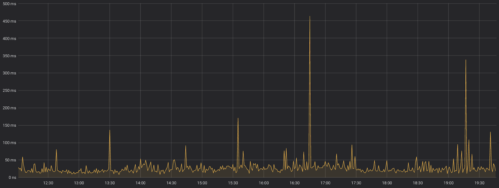
You can clearly see that the baseline response time is around ~20-30 ms. However, we can also see periodic spikes around ~50-100 ms, with peaks up to ~350-450 ms! After a bit of investigation, we concluded that most (although not all) of the spikes were caused by the GC kicking in at the wrong time.

The work I did in the gc-disable branch aims to fix this problem by introducing two new features to the gc module:

• gc.disable(), which previously only inhibited the execution of finalizers without actually touching the GC, now disables the GC major collections. After a call to it, you will see the memory usage grow indefinitely.
• gc.collect_step() is a new function which you can use to manually execute a single incremental GC collection step.

It is worth to specify that gc.disable() disables only the major collections, while minor collections still runs. Moreover, thanks to the JIT's virtuals, many objects with a short and predictable lifetime are not allocated at all. The end result is that most objects with short lifetime are still collected as usual, so the impact of gc.disable() on memory growth is not as bad as it could sound.

Combining these two functions, it is possible to take control of the GC to make sure it runs only when it is acceptable to do so. For an example of usage, you can look at the implementation of a custom GC inside pypytools. The peculiarity is that it also defines a "with nogc():" context manager which you can use to mark performance-critical sections where the GC is not allowed to run.

The following chart compares the behavior of the default PyPy GC and the new custom GC, after a careful placing of nogc() sections:


The yellow line is the same as before, while the purple line shows the new system: almost all spikes have gone, and the baseline performance is about 10% better. There is still one spike towards the end, but after some investigation we concluded that it was not caused by the GC.

Note that this does not mean that the whole program became magically faster: we simply moved the GC pauses in some other place which is not shown in the graph: in this specific use case this technique was useful because it allowed us to shift the GC work in places where pauses are more acceptable.

All in all, a pretty big success, I think. These functionalities are already available in the nightly builds of PyPy, and will be included in the next release: take this as a New Year present :)

Antonio Cuni and the PyPy team

This is a tutorial style post that walks through using the RPython translation toolchain to create a REPL that executes basic math expressions.

We will do that by scanning the user's input into tokens, compiling those tokens into bytecode and running that bytecode in our own virtual machine. Don't worry if that sounds horribly complicated, we are going to explain it step by step.

This post is a bit of a diversion while on my journey to create a compliant lox implementation using the RPython translation toolchain. The majority of this work is a direct RPython translation of the low level C guide from Bob Nystrom (@munificentbob) in the excellent book craftinginterpreters.com specifically the chapters 14 – 17.

The road ahead

As this post is rather long I'll break it into a few major sections. In each section we will have something that translates with RPython, and at the end it all comes together.

• REPL
• Virtual Machine
• Scanning the source
• Compiling Expressions
• End to end

A REPL

So if you're a Python programmer you might be thinking this is pretty trivial right?

I mean if we ignore input errors, injection attacks etc couldn't we just do something like this:

"""
A pure python REPL that can parse simple math expressions
"""
while True:
    print(eval(raw_input("> ")))

Well it does appear to do the trick:

$ python2 section-1-repl/main.py
> 3 + 4 * ((1.0/(2 * 3 * 4)) + (1.0/(4 * 5 * 6)) - (1.0/(6 * 7 * 8)))
3.1880952381

So can we just ask RPython to translate this into a binary that runs magically faster?

Let's see what happens. We need to add two functions for RPython to get its bearings (entry_point and target) and call the file targetXXX:

targetrepl1.py

def repl():
    while True:
        print eval(raw_input('> '))


def entry_point(argv):
    repl()
    return 0


def target(driver, *args):
    return entry_point, None

Which at translation time gives us this admonishment that accurately tells us we are trying to call a Python built-in raw_input that is unfortunately not valid RPython.

$ rpython ./section-1-repl/targetrepl1.py
...SNIP...
[translation:ERROR] AnnotatorError: 

object with a __call__ is not RPython: <built-in function raw_input>
Processing block:
 block@18 is a <class 'rpython.flowspace.flowcontext.SpamBlock'> 
 in (target1:2)repl 
 containing the following operations: 
       v0 = simple_call((builtin_function raw_input), ('> ')) 
       v1 = simple_call((builtin_function eval), v0) 
       v2 = str(v1) 
       v3 = simple_call((function rpython_print_item), v2) 
       v4 = simple_call((function rpython_print_newline)) 

Ok so we can't use raw_input or eval but that doesn't faze us. Let's get the input from a stdin stream and just print it out (no evaluation).

targetrepl2.py

from rpython.rlib import rfile

LINE_BUFFER_LENGTH = 1024


def repl(stdin):
    while True:
        print "> ",
        line = stdin.readline(LINE_BUFFER_LENGTH)
        print line


def entry_point(argv):
    stdin, stdout, stderr = rfile.create_stdio()
    try:
        repl(stdin)
    except:
        return 0


def target(driver, *args):
    return entry_point, None

Translate targetrepl2.py – we can add an optimization level if we are so inclined:

$ rpython --opt=2 section-1-repl/targetrepl2.py
...SNIP...
[Timer] Timings:
[Timer] annotate                       ---  1.2 s
[Timer] rtype_lltype                   ---  0.9 s
[Timer] backendopt_lltype              ---  0.6 s
[Timer] stackcheckinsertion_lltype     ---  0.0 s
[Timer] database_c                     --- 15.0 s
[Timer] source_c                       ---  1.6 s
[Timer] compile_c                      ---  1.9 s
[Timer] =========================================
[Timer] Total:                         --- 21.2 s

No errors!? Let's try it out:

$ ./target2-c 
1 + 2
>  1 + 2

^C

Ahh our first success – let's quickly deal with the flushing fail by using the stdout stream directly as well. Let's print out the input in quotes:

from rpython.rlib import rfile

LINE_BUFFER_LENGTH = 1024


def repl(stdin, stdout):
    while True:
        stdout.write("> ")
        line = stdin.readline(LINE_BUFFER_LENGTH)
        print '"%s"' % line.strip()


def entry_point(argv):
    stdin, stdout, stderr = rfile.create_stdio()
    try:
        repl(stdin, stdout)
    except:
        pass
    return 0


def target(driver, *args):
    return entry_point, None

Translation works, and the test run too:

$ ./target3-c 
> hello this seems better
"hello this seems better"
> ^C

So we are in a good place with taking user input and printing output... What about the whole math evaluation thing we were promised? For that we are can probably leave our RPython REPL behind for a while and connect it up at the end.

A virtual machine

A virtual machine is the execution engine of our basic math interpreter. It will be very simple, only able to do simple tasks like addition. I won't go into any depth to describe why we want a virtual machine, but it is worth noting that many languages including Java and Python make this decision to compile to an intermediate bytecode representation and then execute that with a virtual machine. Alternatives are compiling directly to native machine code like (earlier versions of) the V8 JavaScript engine, or at the other end of the spectrum executing an abstract syntax tree – which is what the Truffle approach to building VMs is based on.

We are going to keep things very simple. We will have a stack where we can push and pop values, we will only support floats, and our VM will only implement a few very basic operations.

OpCodes

In fact our entire instruction set is:

OP_CONSTANT
OP_RETURN
OP_NEGATE
OP_ADD
OP_SUBTRACT
OP_MULTIPLY
OP_DIVIDE

Since we are targeting RPython we can't use the nice enum module from the Python standard library, so instead we just define a simple class with class attributes.

We should start to get organized, so we will create a new file opcodes.py and add this:

class OpCode:
    OP_CONSTANT = 0
    OP_RETURN = 1
    OP_NEGATE = 2
    OP_ADD = 3
    OP_SUBTRACT = 4
    OP_MULTIPLY = 5
    OP_DIVIDE = 6

Chunks

To start with we need to get some infrastructure in place before we write the VM engine.

Following craftinginterpreters.com we start with a Chunk object which will represent our bytecode. In RPython we have access to Python-esq lists so our code object will just be a list of OpCode values – which are just integers. A list of ints, couldn't get much simpler.

section-2-vm/chunk.py

class Chunk:
    code = None

    def __init__(self):
        self.code = []

    def write_chunk(self, byte):
        self.code.append(byte)

    def disassemble(self, name):
        print "== %s ==\n" % name
        i = 0
        while i < len(self.code):
            i = disassemble_instruction(self, i)

From here on I'll only present minimal snippets of code instead of the whole lot, but I'll link to the repository with the complete example code. For example the various debugging including disassemble_instruction isn't particularly interesting to include verbatim. See the github repo for full details

We need to check that we can create a chunk and disassemble it. The quickest way to do this is to use Python during development and debugging then every so often try to translate it.

Getting the disassemble part through the RPython translator was a hurdle for me as I quickly found that many str methods such as format are not supported, and only very basic % based formatting is supported. I ended up creating helper functions for string manipulation such as:

def leftpad_string(string, width, char=" "):
    l = len(string)
    if l > width:
        return string
    return char * (width - l) + string

Let's write a new entry_point that creates and disassembles a chunk of bytecode. We can set the target output name to vm1 at the same time:

targetvm1.py

def entry_point(argv):
    bytecode = Chunk()
    bytecode.write_chunk(OpCode.OP_ADD)
    bytecode.write_chunk(OpCode.OP_RETURN)
    bytecode.disassemble("hello world")
    return 0

def target(driver, *args):
    driver.exe_name = "vm1"
    return entry_point, None

Running this isn't going to be terribly interesting, but it is always nice to know that it is doing what you expect:

$ ./vm1 
== hello world ==

0000 OP_ADD       
0001 OP_RETURN    

Chunks of data

Ref: https://www.craftinginterpreters.com/chunks-of-bytecode.html#constants

So our bytecode is missing a very crucial element – the values to operate on!

As with the bytecode we can store these constant values as part of the chunk directly in a list. Each chunk will therefore have a constant data component, and a code component.

Edit the chunk.py file and add the new instance attribute constants as an empty list, and a new method add_constant.

    def add_constant(self, value):
        self.constants.append(value)
        return len(self.constants) - 1

Now to use this new capability we can modify our example chunk to write in some constants before the OP_ADD:

    bytecode = Chunk()
    constant = bytecode.add_constant(1.0)
    bytecode.write_chunk(OpCode.OP_CONSTANT)
    bytecode.write_chunk(constant)

    constant = bytecode.add_constant(2.0)
    bytecode.write_chunk(OpCode.OP_CONSTANT)
    bytecode.write_chunk(constant)

    bytecode.write_chunk(OpCode.OP_ADD)
    bytecode.write_chunk(OpCode.OP_RETURN)

    bytecode.disassemble("adding constants")

Which still translates with RPython and when run gives us the following disassembled bytecode:

== adding constants ==

0000 OP_CONSTANT  (00)        '1'
0002 OP_CONSTANT  (01)        '2'
0004 OP_ADD       
0005 OP_RETURN

We won't go down the route of serializing the bytecode to disk, but this bytecode chunk (including the constant data) could be saved and executed on our VM later – like a Java .class file. Instead we will pass the bytecode directly to our VM after we've created it during the compilation process.

Emulation

So those four instructions of bytecode combined with the constant value mapping 00 -> 1.0 and 01 -> 2.0 describes individual steps for our virtual machine to execute. One major point in favor of defining our own bytecode is we can design it to be really simple to execute – this makes the VM really easy to implement.

As I mentioned earlier this virtual machine will have a stack, so let's begin with that. Now the stack is going to be a busy little beast – as our VM takes instructions like OP_ADD it will pop off the top two values from the stack, and push the result of adding them together back onto the stack. Although dynamically resizing Python lists are marvelous, they can be a little slow. RPython can take advantage of a constant sized list which doesn't make our code much more complicated.

To do this we will define a constant sized list and track the stack_top directly. Note how we can give the RPython translator hints by adding assertions about the state that the stack_top will be in.

class VM(object):
    STACK_MAX_SIZE = 256
    stack = None
    stack_top = 0

    def __init__(self):
        self._reset_stack()

    def _reset_stack(self):
        self.stack = [0] * self.STACK_MAX_SIZE
        self.stack_top = 0

    def _stack_push(self, value):
        assert self.stack_top < self.STACK_MAX_SIZE
        self.stack[self.stack_top] = value
        self.stack_top += 1

    def _stack_pop(self):
        assert self.stack_top >= 0
        self.stack_top -= 1
        return self.stack[self.stack_top]

    def _print_stack(self):
        print "         ",
        if self.stack_top <= 0:
            print "[]",
        else:
            for i in range(self.stack_top):
                print "[ %s ]" % self.stack[i],
        print

Now we get to the main event, the hot loop, the VM engine. Hope I haven't built it up to much, it is actually really simple! We loop until the instructions tell us to stop (OP_RETURN), and dispatch to other simple methods based on the instruction.

    def _run(self):
        while True:
            instruction = self._read_byte()

            if instruction == OpCode.OP_RETURN:
                print "%s" % self._stack_pop()
                return InterpretResultCode.INTERPRET_OK
            elif instruction == OpCode.OP_CONSTANT:
                constant = self._read_constant()
                self._stack_push(constant)
            elif instruction == OpCode.OP_ADD:
                self._binary_op(self._stack_add)    

Now the _read_byte method will have to keep track of which instruction we are up to. So add an instruction pointer (ip) to the VM with an initial value of 0. Then _read_byte is simply getting the next bytecode (int) from the chunk's code:

    def _read_byte(self):
        instruction = self.chunk.code[self.ip]
        self.ip += 1
        return instruction

If the instruction is OP_CONSTANT we take the constant's address from the next byte of the chunk's code, retrieve that constant value and add it to the VM's stack.

    def _read_constant(self):
        constant_index = self._read_byte()
        return self.chunk.constants[constant_index]

Finally our first arithmetic operation OP_ADD, what it has to achieve doesn't require much explanation: pop two values from the stack, add them together, push the result. But since a few operations all have the same template we introduce a layer of indirection – or abstraction – by introducing a reusable _binary_op helper method.

    @specialize.arg(1)
    def _binary_op(self, operator):
        op2 = self._stack_pop()
        op1 = self._stack_pop()
        result = operator(op1, op2)
        self._stack_push(result)

    @staticmethod
    def _stack_add(op1, op2):
        return op1 + op2

Note we tell RPython to specialize _binary_op on the first argument. This causes RPython to make a copy of _binary_op for every value of the first argument passed, which means that each copy contains a call to a particular operator, which can then be inlined.

To be able to run our bytecode the only thing left to do is to pass in the chunk and call _run():

    def interpret_chunk(self, chunk):
        if self.debug_trace:
            print "== VM TRACE =="
        self.chunk = chunk
        self.ip = 0
        try:
            result = self._run()
            return result
        except:
            return InterpretResultCode.INTERPRET_RUNTIME_ERROR

targetvm3.py connects the pieces:

def entry_point(argv):
    bytecode = Chunk()
    constant = bytecode.add_constant(1)
    bytecode.write_chunk(OpCode.OP_CONSTANT)
    bytecode.write_chunk(constant)
    constant = bytecode.add_constant(2)
    bytecode.write_chunk(OpCode.OP_CONSTANT)
    bytecode.write_chunk(constant)
    bytecode.write_chunk(OpCode.OP_ADD)
    bytecode.write_chunk(OpCode.OP_RETURN)

    vm = VM()
    vm.interpret_chunk(bytecode)

    return 0

I've added some trace debugging so we can see what the VM and stack is doing.

The whole thing translates with RPython, and when run gives us:

./vm3
== VM TRACE ==
          []
0000 OP_CONSTANT  (00)        '1'
          [ 1 ]
0002 OP_CONSTANT  (01)        '2'
          [ 1 ] [ 2 ]
0004 OP_ADD       
          [ 3 ]
0005 OP_RETURN    
3

Yes we just computed the result of 1+2. Pat yourself on the back.

At this point it is probably valid to check that the translated executable is actually faster than running our program directly in Python. For this trivial example under Python2/pypy this targetvm3.py file runs in the 20ms – 90ms region, and the compiled vm3 runs in <5ms. Something useful must be happening during the translation.

I won't go through the code adding support for our other instructions as they are very similar and straightforward. Our VM is ready to execute our chunks of bytecode, but we haven't yet worked out how to take the entered expression and turn that into this simple bytecode. This is broken into two steps, scanning and compiling.

Scanning the source

All the source for this section can be found in section-3-scanning.

The job of the scanner is to take the raw expression string and transform it into a sequence of tokens. This scanning step will strip out whitespace and comments, catch errors with invalid token and tokenize the string. For example the input "( 1 + 2 ) would get tokenized into LEFT_PAREN, NUMBER(1), PLUS, NUMBER(2), RIGHT_PAREN.

As with our OpCodes we will just define a simple Python class to define an int for each type of token:

class TokenTypes:
    ERROR = 0
    EOF = 1
    LEFT_PAREN = 2
    RIGHT_PAREN = 3
    MINUS = 4
    PLUS = 5
    SLASH = 6
    STAR = 7
    NUMBER = 8

A token has to keep some other information as well – keeping track of the location and length of the token will be helpful for error reporting. The NUMBER token clearly needs some data about the value it is representing: we could include a copy of the source lexeme (e.g. the string 2.0), or parse the value and store that, or – what we will do in this blog – use the location and length information as pointers into the original source string. Every token type (except perhaps ERROR) will use this simple data structure:

class Token(object):

    def __init__(self, start, length, token_type):
        self.start = start
        self.length = length
        self.type = token_type

Our soon to be created scanner will create these Token objects which refer back to addresses in some source. If the scanner sees the source "( 1 + 2.0 )" it would emit the following tokens:

Token(0, 1, TokenTypes.LEFT_PAREN)
Token(2, 1, TokenTypes.NUMBER)
Token(4, 1, TokenTypes.PLUS)
Token(6, 3, TokenTypes.NUMBER)
Token(10, 1, TokenTypes.RIGHT_PAREN)

Scanner

Let's walk through the scanner implementation method by method. The scanner will take the source and pass through it once, creating tokens as it goes.

class Scanner(object):

    def __init__(self, source):
        self.source = source
        self.start = 0
        self.current = 0

The start and current variables are character indices in the source string that point to the current substring being considered as a token.

For example in the string "(51.05+2)" while we are tokenizing the number 51.05 we will have start pointing at the 5, and advance current character by character until the character is no longer part of a number. Midway through scanning the number the start and current values might point to 1 and 4 respectively:

0	1	2	3	4	5	6	7	8
"("	"5"	"1"	"."	"0"	"5"	"+"	"2"	")"
	^			^

From current=4 the scanner peeks ahead and sees that the next character (5) is a digit, so will continue to advance.

0	1	2	3	4	5	6	7	8
"("	"5"	"1"	"."	"0"	"5"	"+"	"2"	")"
	^				^

When the scanner peeks ahead and sees the "+" it will create the number token and emit it. The method that carry's out this tokenizing is _number:

    def _number(self):
        while self._peek().isdigit():
            self.advance()

        # Look for decimal point
        if self._peek() == '.' and self._peek_next().isdigit():
            self.advance()
            while self._peek().isdigit():
                self.advance()

        return self._make_token(TokenTypes.NUMBER)

It relies on a few helpers to look ahead at the upcoming characters:

    def _peek(self):
        if self._is_at_end():
            return '\0'
        return self.source[self.current]

    def _peek_next(self):
        if self._is_at_end():
            return '\0'
        return self.source[self.current+1]

    def _is_at_end(self):
        return len(self.source) == self.current

If the character at current is still part of the number we want to call advance to move on by one character.

    def advance(self):
        self.current += 1
        return self.source[self.current - 1]

Once the isdigit() check fails in _number() we call _make_token() to emit the token with the NUMBER type.

    def _make_token(self, token_type):
        return Token(
            start=self.start,
            length=(self.current - self.start),
            token_type=token_type
        )

Note again that the token is linked to an index address in the source, rather than including the string value.

Our scanner is pull based, a token will be requested via scan_token. First we skip past whitespace and depending on the characters emit the correct token:

    def scan_token(self):
        # skip any whitespace
        while True:
            char = self._peek()
            if char in ' \r\t\n':
                self.advance()
            break

        self.start = self.current

        if self._is_at_end():
            return self._make_token(TokenTypes.EOF)

        char = self.advance()

        if char.isdigit():
            return self._number()

        if char == '(':
            return self._make_token(TokenTypes.LEFT_PAREN)
        if char == ')':
            return self._make_token(TokenTypes.RIGHT_PAREN)
        if char == '-':
            return self._make_token(TokenTypes.MINUS)
        if char == '+':
            return self._make_token(TokenTypes.PLUS)
        if char == '/':
            return self._make_token(TokenTypes.SLASH)
        if char == '*':
            return self._make_token(TokenTypes.STAR)

        return ErrorToken("Unexpected character", self.current)

If this was a real programming language we were scanning, this would be the point where we add support for different types of literals and any language identifiers/reserved words.

At some point we will need to parse the literal value for our numbers, but we leave that job for some later component, for now we'll just add a get_token_string helper. To make sure that RPython is happy to index arbitrary slices of source we add range assertions:

    def get_token_string(self, token):
        if isinstance(token, ErrorToken):
            return token.message
        else:
            end_loc = token.start + token.length
            assert end_loc < len(self.source)
            assert end_loc > 0
            return self.source[token.start:end_loc]

A simple entry point can be used to test our scanner with a hard coded source string:

targetscanner1.py

from scanner import Scanner, TokenTypes, TokenTypeToName


def entry_point(argv):

    source = "(   1   + 2.0 )"

    scanner = Scanner(source)
    t = scanner.scan_token()
    while t.type != TokenTypes.EOF and t.type != TokenTypes.ERROR:
        print TokenTypeToName[t.type],
        if t.type == TokenTypes.NUMBER:
            print "(%s)" % scanner.get_token_string(t),
        print
        t = scanner.scan_token()
    return 0

RPython didn't complain, and lo it works:

$ ./scanner1 
LEFT_PAREN
NUMBER (1)
PLUS
NUMBER (2.0)
RIGHT_PAREN

Let's connect our REPL to the scanner.

targetscanner2.py

from rpython.rlib import rfile
from scanner import Scanner, TokenTypes, TokenTypeToName

LINE_BUFFER_LENGTH = 1024


def repl(stdin, stdout):
    while True:
        stdout.write("> ")
        source = stdin.readline(LINE_BUFFER_LENGTH)

        scanner = Scanner(source)
        t = scanner.scan_token()
        while t.type != TokenTypes.EOF and t.type != TokenTypes.ERROR:
            print TokenTypeToName[t.type],
            if t.type == TokenTypes.NUMBER:
                print "(%s)" % scanner.get_token_string(t),
            print
            t = scanner.scan_token()


def entry_point(argv):
    stdin, stdout, stderr = rfile.create_stdio()
    try:
        repl(stdin, stdout)
    except:
        pass
    return 0

With our REPL hooked up we can now scan tokens from arbitrary input:

$ ./scanner2
> (3 *4) - -3
LEFT_PAREN
NUMBER (3)
STAR
NUMBER (4)
RIGHT_PAREN
MINUS
MINUS
NUMBER (3)
> ^C

Compiling expressions

References

• https://www.craftinginterpreters.com/compiling-expressions.html
• https://effbot.org/zone/simple-top-down-parsing.htm

The final piece is to turn this sequence of tokens into our low level bytecode instructions for the virtual machine to execute. Buckle up, we are about to write us a compiler.

Our compiler will take a single pass over the tokens using Vaughan Pratt’s parsing technique, and output a chunk of bytecode – if we do it right it will be compatible with our existing virtual machine.

Remember the bytecode we defined above is really simple – by relying on our stack we can transform a nested expression into a sequence of our bytecode operations.

To make this more concrete let's go through by hand translating an expression into bytecode.

Our source expression:

(3 + 2) - (7 * 2)

If we were to make an abstract syntax tree we'd get something like this:

Now if we start at the first sub expression (3+2) we can clearly note from the first open bracket that we must see a close bracket, and that the expression inside that bracket must be valid on its own. Not only that but regardless of the inside we know that the whole expression still has to be valid. Let's focus on this first bracketed expression, let our attention recurse into it so to speak.

This gives us a much easier problem – we just want to get our virtual machine to compute 3 + 2. In this bytecode dialect we would load the two constants, and then add them with OP_ADD like so:

OP_CONSTANT  (00) '3.000000'
OP_CONSTANT  (01) '2.000000'
OP_ADD

The effect of our vm executing these three instructions is that sitting pretty at the top of the stack is the result of the addition. Winning.

Jumping back out from our bracketed expression, our next token is MINUS, at this point we have a fair idea that it must be used in an infix position. In fact whatever token followed the bracketed expression it must be a valid infix operator, if not the expression is over or had a syntax error.

Assuming the best from our user (naive), we handle MINUS the same way we handled the first PLUS. We've already got the first operand on the stack, now we compile the right operand and then write out the bytecode for OP_SUBTRACT.

The right operand is another simple three instructions:

OP_CONSTANT  (02) '7.000000'
OP_CONSTANT  (03) '2.000000'
OP_MULTIPLY

Then we finish our top level binary expression and write a OP_RETURN to return the value at the top of the stack as the execution's result. Our final hand compiled program is:

OP_CONSTANT  (00) '3.000000'
OP_CONSTANT  (01) '2.000000'
OP_ADD
OP_CONSTANT  (02) '7.000000'
OP_CONSTANT  (03) '2.000000'
OP_MULTIPLY
OP_SUBTRACT
OP_RETURN

Ok that wasn't so hard was it? Let's try make our code do that.

We define a parser object which will keep track of where we are, and whether things have all gone horribly wrong:

class Parser(object):
    def __init__(self):
        self.had_error = False
        self.panic_mode = False
        self.current = None
        self.previous = None

The compiler will also be a class, we'll need one of our Scanner instances to pull tokens from, and since the output is a bytecode Chunk let's go ahead and make one of those in our compiler initializer:

class Compiler(object):

    def __init__(self, source):
        self.parser = Parser()
        self.scanner = Scanner(source)
        self.chunk = Chunk()

Since we have this (empty) chunk of bytecode we will make a helper method to add individual bytes. Every instruction will pass from our compiler into an executable program through this simple .

    def emit_byte(self, byte):
        self.current_chunk().write_chunk(byte)

To quote from Bob Nystrom on the Pratt parsing technique:

the implementation is a deceptively-simple handful of deeply intertwined code

I don't actually think I can do justice to this section. Instead I suggest reading his treatment in Pratt Parsers: Expression Parsing Made Easy which explains the magic behind the parsing component. Our only major difference is instead of creating an AST we are going to directly emit bytecode for our VM.

Now that I've absolved myself from taking responsibility in explaining this somewhat tricky concept, I'll discuss some of the code from compiler.py, and walk through what happens for a particular rule.

I'll jump straight to the juicy bit the table of parse rules. We define a ParseRule for each token, and each rule comprises:

• an optional handler for when the token is as a prefix (e.g. the minus in (-2)),
• an optional handler for whet the token is used infix (e.g. the slash in 2/47)
• a precedence value (a number that determines what is of higher precedence)

rules = [
    ParseRule(None,              None,            Precedence.NONE),   # ERROR
    ParseRule(None,              None,            Precedence.NONE),   # EOF
    ParseRule(Compiler.grouping, None,            Precedence.CALL),   # LEFT_PAREN
    ParseRule(None,              None,            Precedence.NONE),   # RIGHT_PAREN
    ParseRule(Compiler.unary,    Compiler.binary, Precedence.TERM),   # MINUS
    ParseRule(None,              Compiler.binary, Precedence.TERM),   # PLUS
    ParseRule(None,              Compiler.binary, Precedence.FACTOR), # SLASH
    ParseRule(None,              Compiler.binary, Precedence.FACTOR), # STAR
    ParseRule(Compiler.number,   None,            Precedence.NONE),   # NUMBER
]

These rules really are the magic of our compiler. When we get to a particular token such as MINUS we see if it is an infix operator and if so we've gone and got its first operand ready. At all times we rely on the relative precedence; consuming everything with higher precedence than the operator we are currently evaluating.

In the expression:

2 + 3 * 4

The * has higher precedence than the +, so 3 * 4 will be parsed together as the second operand to the first infix operator (the +) which follows the BEDMAS order of operations I was taught at high school.

To encode these precedence values we make another Python object moonlighting as an enum:

class Precedence(object):
    NONE = 0
    DEFAULT = 1
    TERM = 2        # + -
    FACTOR = 3      # * /
    UNARY = 4       # ! - +
    CALL = 5        # ()
    PRIMARY = 6

What happens in our compiler when turning -2.0 into bytecode? Assume we've just pulled the token MINUS from the scanner. Every expression has to start with some type of prefix – whether that is:

• a bracket group (,
• a number 2,
• or a prefix unary operator -.

Knowing that, our compiler assumes there is a prefix handler in the rule table – in this case it points us at the unary handler.

    def parse_precedence(self, precedence):
        # parses any expression of a given precedence level or higher
        self.advance()
        prefix_rule = self._get_rule(self.parser.previous.type).prefix
        prefix_rule(self)

unary is called:

    def unary(self):
        op_type = self.parser.previous.type
        # Compile the operand
        self.parse_precedence(Precedence.UNARY)
        # Emit the operator instruction
        if op_type == TokenTypes.MINUS:
            self.emit_byte(OpCode.OP_NEGATE)

Here – before writing the OP_NEGATE opcode we recurse back into parse_precedence to ensure that whatever follows the MINUS token is compiled – provided it has higher precedence than unary – e.g. a bracketed group. Crucially at run time this recursive call will ensure that the result is left on top of our stack. Armed with this knowledge, the unary method just has to emit a single byte with the OP_NEGATE opcode.

Test compilation

Now we can test our compiler by outputting disassembled bytecode of our user entered expressions. Create a new entry_point targetcompiler:

from rpython.rlib import rfile
from compiler import Compiler

LINE_BUFFER_LENGTH = 1024


def entry_point(argv):
    stdin, stdout, stderr = rfile.create_stdio()

    try:
        while True:
            stdout.write("> ")
            source = stdin.readline(LINE_BUFFER_LENGTH)
            compiler = Compiler(source, debugging=True)
            compiler.compile()
    except:
        pass
    return 0

Translate it and test it out:

$ ./compiler1 
> (2/4 + 1/2)
== code ==

0000 OP_CONSTANT  (00) '2.000000'
0002 OP_CONSTANT  (01) '4.000000'
0004 OP_DIVIDE    
0005 OP_CONSTANT  (02) '1.000000'
0007 OP_CONSTANT  (00) '2.000000'
0009 OP_DIVIDE    
0010 OP_ADD       
0011 OP_RETURN

Now if you've made it this far you'll be eager to finally connect everything together by executing this bytecode with the virtual machine.

End to end

All the pieces slot together rather easily at this point, create a new file targetcalc.py and define our entry point:

from rpython.rlib import rfile
from compiler import Compiler
from vm import VM

LINE_BUFFER_LENGTH = 4096


def entry_point(argv):
    stdin, stdout, stderr = rfile.create_stdio()
    vm = VM()
    try:
        while True:
            stdout.write("> ")
            source = stdin.readline(LINE_BUFFER_LENGTH)
            if source:
                compiler = Compiler(source, debugging=False)
                compiler.compile()
                vm.interpret_chunk(compiler.chunk)
    except:
        pass
    return 0


def target(driver, *args):
    driver.exe_name = "calc"
    return entry_point, None

Let's try catch it out with a double negative:

$ ./calc 
> 2--3
== VM TRACE ==
          []
0000 OP_CONSTANT  (00) '2.000000'
          [ 2.000000 ]
0002 OP_CONSTANT  (01) '3.000000'
          [ 2.000000 ] [ 3.000000 ]
0004 OP_NEGATE    
          [ 2.000000 ] [ -3.000000 ]
0005 OP_SUBTRACT  
          [ 5.000000 ]
0006 OP_RETURN    
5.000000

Ok well let's evaluate the first 50 terms of the Nilakantha Series:

$ ./calc
> 3 + 4 * ((1/(2 * 3 * 4)) + (1/(4 * 5 * 6)) - (1/(6 * 7 * 8)) + (1/(8 * 9 * 10)) - (1/(10 * 11 * 12)) + (1/(12 * 13 * 14)) - (1/(14 * 15 * 16)) + (1/(16 * 17 * 18)) - (1/(18 * 19 * 20)) + (1/(20 * 21 * 22)) - (1/(22 * 23 * 24)) + (1/(24 * 25 * 26)) - (1/(26 * 27 * 28)) + (1/(28 * 29 * 30)) - (1/(30 * 31 * 32)) + (1/(32 * 33 * 34)) - (1/(34 * 35 * 36)) + (1/(36 * 37 * 38)) - (1/(38 * 39 * 40)) + (1/(40 * 41 * 42)) - (1/(42 * 43 * 44)) + (1/(44 * 45 * 46)) - (1/(46 * 47 * 48)) + (1/(48 * 49 * 50)) - (1/(50 * 51 * 52)) + (1/(52 * 53 * 54)) - (1/(54 * 55 * 56)) + (1/(56 * 57 * 58)) - (1/(58 * 59 * 60)) + (1/(60 * 61 * 62)) - (1/(62 * 63 * 64)) + (1/(64 * 65 * 66)) - (1/(66 * 67 * 68)) + (1/(68 * 69 * 70)) - (1/(70 * 71 * 72)) + (1/(72 * 73 * 74)) - (1/(74 * 75 * 76)) + (1/(76 * 77 * 78)) - (1/(78 * 79 * 80)) + (1/(80 * 81 * 82)) - (1/(82 * 83 * 84)) + (1/(84 * 85 * 86)) - (1/(86 * 87 * 88)) + (1/(88 * 89 * 90)) - (1/(90 * 91 * 92)) + (1/(92 * 93 * 94)) - (1/(94 * 95 * 96)) + (1/(96 * 97 * 98)) - (1/(98 * 99 * 100)) + (1/(100 * 101 * 102)))

== VM TRACE ==
          []
0000 OP_CONSTANT  (00) '3.000000'
          [ 3.000000 ]
0002 OP_CONSTANT  (01) '4.000000'
...SNIP...
0598 OP_CONSTANT  (101) '102.000000'
          [ 3.000000 ] [ 4.000000 ] [ 0.047935 ] [ 1.000000 ] [ 10100.000000 ] [ 102.000000 ]
0600 OP_MULTIPLY  
          [ 3.000000 ] [ 4.000000 ] [ 0.047935 ] [ 1.000000 ] [ 1030200.000000 ]
0601 OP_DIVIDE    
          [ 3.000000 ] [ 4.000000 ] [ 0.047935 ] [ 0.000001 ]
0602 OP_ADD       
          [ 3.000000 ] [ 4.000000 ] [ 0.047936 ]
0603 OP_MULTIPLY  
          [ 3.000000 ] [ 0.191743 ]
0604 OP_ADD       
          [ 3.191743 ]
0605 OP_RETURN    
3.191743

We just executed 605 virtual machine instructions to compute pi to 1dp!

This brings us to the end of this tutorial. To recap we've walked through the whole compilation process: from the user providing an expression string on the REPL, scanning the source string into tokens, parsing the tokens while accounting for relative precedence via a Pratt parser, generating bytecode, and finally executing the bytecode on our own VM. RPython translated what we wrote into C and compiled it, meaning our resulting calc REPL is really fast.

“The world is a thing of utter inordinate complexity and richness and strangeness that is absolutely awesome.”

― Douglas Adams

Many thanks to Bob Nystrom for writing the book that inspired this post, and thanks to Carl Friedrich and Matt Halverson for reviewing.

― Brian (@thorneynzb)